COMP3056 Computer Vision 3 -- Image Stitching

Table of Contents

• Image Stitching
  • Geometric Transformations
    • Basic Transformations
    • Combined Transformation
  • Image Stitching
    • [IMPORTANT] Idea of Stitching
    • Motion Models
    • [IMPORTANT] RANSAC
  • Image Warping
    • [UNDERSTAND] Forward Warping
    • [UNDERSTAND] Inverse Warping
    • [UNDERSTAND] Which one is better - Usually inverse
  • Image Blending
    • [IMPORTANT] Pyramid Blending
    • Detailed Steps:
    • [NOT IMPORTANT] Multiband Blending
  • [IMPORTANT] Recognizing Panoramas

Image Stitching

Geometric Transformations

Basic Transformations

• Translation
• Rotation
• Scale
• Aspect Ratio
• Shear

Combined Transformation

• Euclidean transform = Translation + Rotation (1+2 DOF)
  • 刚体变换/欧氏距离变换- 3 Degree Of Freedom (DOF)
• Similarity transform = Translation + Rotation + Scale (1+2+1 DOF)
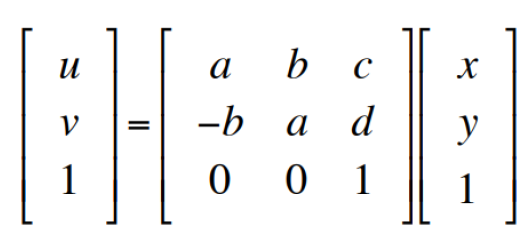
  • 相似变换 - 4 DOF
• Affine transform = Translation + Rotation + Scale + Aspect Ratio + Shear
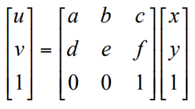
  • 仿射变换 - 6 DOF
• Projective transform - Homogeneous Coordinates
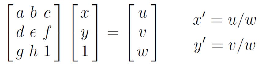
  • 投影变换- 8 DOF

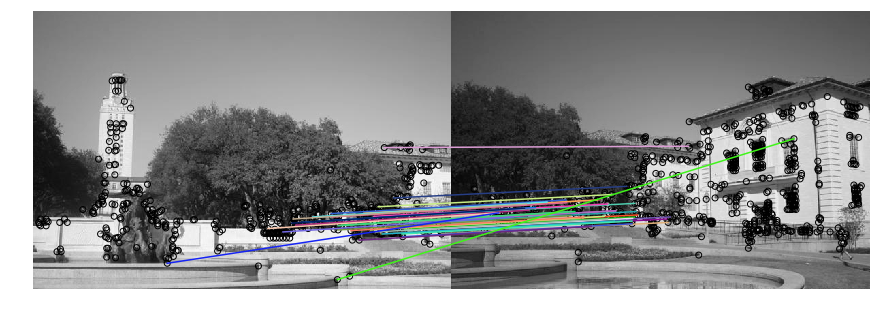
Image Stitching

[IMPORTANT] Idea of Stitching

1. Take a sequence of images from the same position.
   • Rotate the camera about its optical center
   • Or hold the camera and turn the body without changing the position if there are no tripods.
2. To stitch two images: compute transformation between the second image and the first.
   • Extract interest points
   • Find Matches
   • Compute
3. Shift (warp) the second image to overlap with the first.
4. Blend the two together to create a mosaic.
5. If there are more images, repeat step 2 to 4.

Motion Models

• Translation = 2 DOF - 1 Pairs
• Similarity = 4 DOF - 2 Pairs
• Affine = 6 DOF - 3 Pairs
• Projective (Homography) = 8 DOF - 4 Pairs

[IMPORTANT] RANSAC

Random Sample Consensus 随机样本一致性算法

• RANSAC loop for estimating homography

1. Select 4 feature pairs (at random)
2. Compute homography \(H\)(exact)
3. Compute inliers where \(||p_i ', H p_i|| < \varepsilon\)

• Keep the largest set of inliers
• Re-compute least squares H estimate using all of the inliers

The idea of fitting a RANSAC line: Use the biggest set of inliers and do the least-square fit

Image Warping

describe the idea of two warping methods
Change every pixel locations to create a new image (global)
Transform function \(x' = h(x)\)
Source image \(f(x)\)
Transformed image \(g(x') = f(h(x))\)

• Change the domain of image function

[UNDERSTAND] Forward Warping

Send each pixel \(f(x)\) from the original image (RGB value) to the dest image: \(x' = h(x)\) in\(g(x')\)
If pixel lands "between" 2 pixels, then add "contribution" to several neighboring pixels, normalize later (splatting)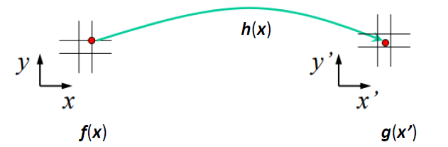

[UNDERSTAND] Inverse Warping

Get each pixel \(g(x')\) from the transformed image to the source image: \(x=h^{-1}(x')\) in \(f(x)\)
If pixel comes from "between" 2 pixels, then resample color value from the interpolated source image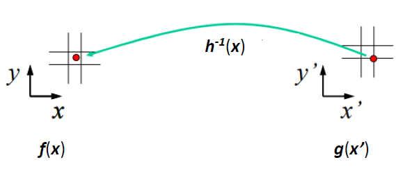

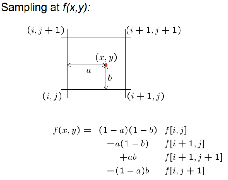
• Possible interpolation filters:
  • Nearest neighbor
  • Bilinear

bilinear

[UNDERSTAND] Which one is better - Usually inverse

https://blog.csdn.net/baoyongshuai1509/article/details/109013703

• Because the result of forward warping might show some holes like gray marks in the figure. That is no pixels are mapped to this position after warping. While some points may fall into the same position in the new map, as shown in the red box below. This is because of the discretization of image pixels. The transform function is usually neither injective nor surjective, so the non-integral value after warping will be rounded off, so not every pixel in the original image will be assigned a pixel value in the new image. Similarly, a single pixel in the new image may correspond to multiple pixels in the original image
• By using inverse warping, this problem can be reduced (interpolation)
• But it is not always possible to get an invertible warp function

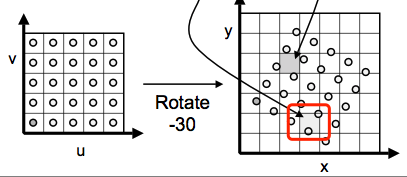
Image Blending

Most of the formulas are not important
blend two images together
Just for knowledge

• Feathering
• Effect of window size
• Alpha Blending

[IMPORTANT] Pyramid Blending

Step Summary:

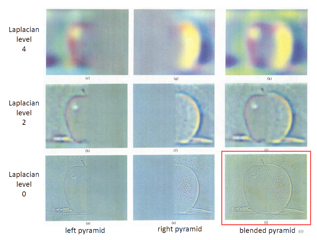
1. Form two Gaussian Pyramids from 2 images
2. Generate their Laplacian Pyramids LA and LB
3. Construct a new Pyramid LS from LA and LB by combining the left half of LA and the right half of LB
4. Reconstruct the blended image from the new Pyramid LS

Detailed Steps:

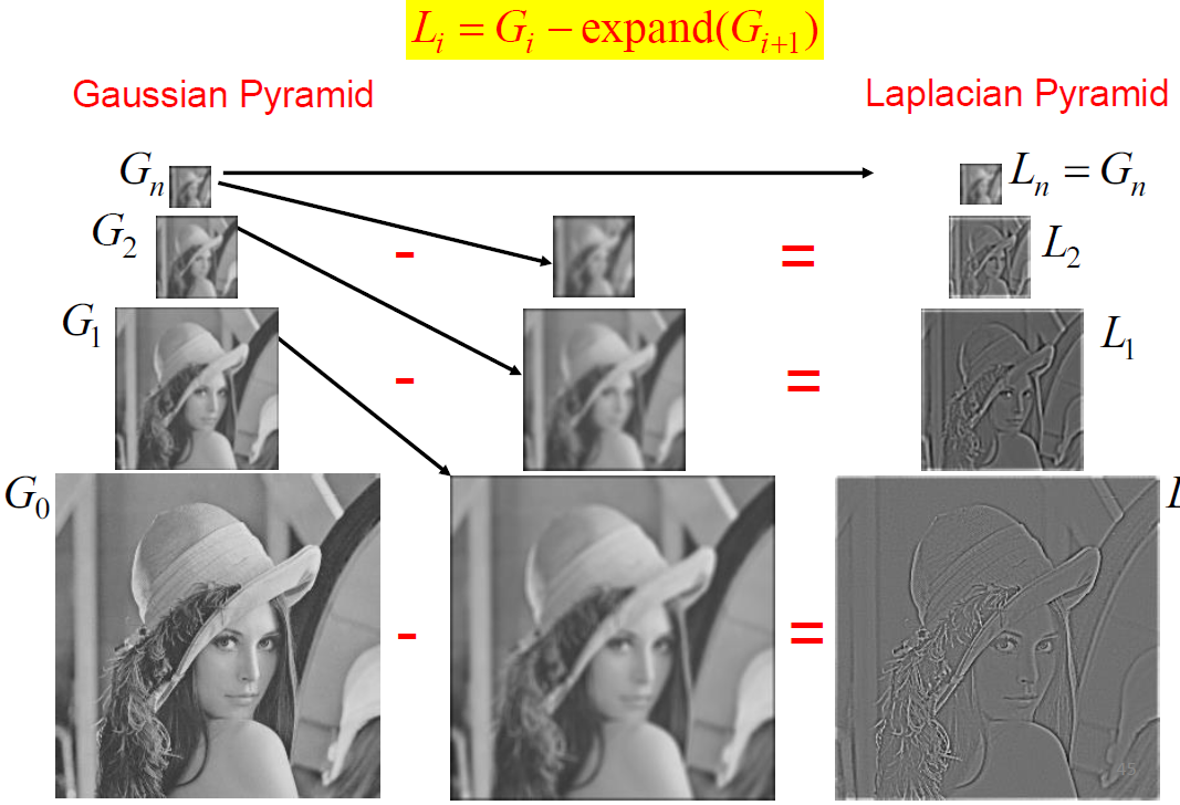
1. Forming a Gaussian Pyramid
   • Start with the original image \(G_0\)
   • Perform a Gaussian filtering about each pixel, down sampling so that the result is a reduced image of half the size in each dimension.
   • Do this all the way up the pyramid.
   • \(G_I = REDUCE(G_{i-1})\)
2. Making the Laplacians
   • Subtract each level of the pyramid from the next lower one
   • Perform an interpolation process to do the subtraction because of different sizes in different levels.
     • Interpolate new samples between those of a given image to make it big enough to subtract.
     • The operation is called EXPAND

gaussian pyramid

3. Forming the New Pyramid
   • Laplacian pyramids LA and LB are constructed for images A and B, respectively.
   • A third Laplacian pyramid LS is constructed by copying nodes from the left half of LA to the corresponding nodes of LS and nodes from the right half of LB to the right half of LS.
   • Nodes along the center line are set equal to the average of corresponding LA and LB nodes
4. Using the New Laplacian Pyramid
   • Use the new Laplacian pyramid with the reverse of how it was created to create a Gaussian pyramid.
   • \(G_i = L_i + expand(G_{i+1})\)
   • The lowest level gives the result

完整过程图示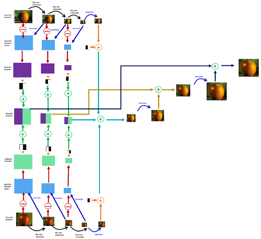

[NOT IMPORTANT] Multiband Blending

• Decompose the image into multi-band frequency
• Blend each band appropriately
• At low frequencies, blend slowly
  • Image regions that are “smooth”
• At high frequencies, blend quickly
  • Image regions have a lot of pixel intensity variation

Steps:

1. Compute Laplacian pyramid of images and mask.
2. Create blended image at each level of pyramid.
3. Reconstruct complete image.

[IMPORTANT] Recognizing Panoramas

Steps:

1. Extract SIFT points, descriptors from all images
2. Find K-nearest neighbors for each point (K=4)
3. For each image
   1. Select M candidate matching images by counting matched keypoints (M=6)
   2. Solve homography \(H_{ij}\) for each matched image
   3. Decide if match is valid \((n_i > 8 + 0.3 n_f)\)

Then we have matched pairs of images

4. Make a graph of matched pairs to find connected components of the graph
5. For each connected component
   1. Solve for rotation and f (camera parameters)
   2. Project to a surface (plane, cylinder, or sphere)
   3. Render with multiband blending